Step-by-step guide

1 Get an account

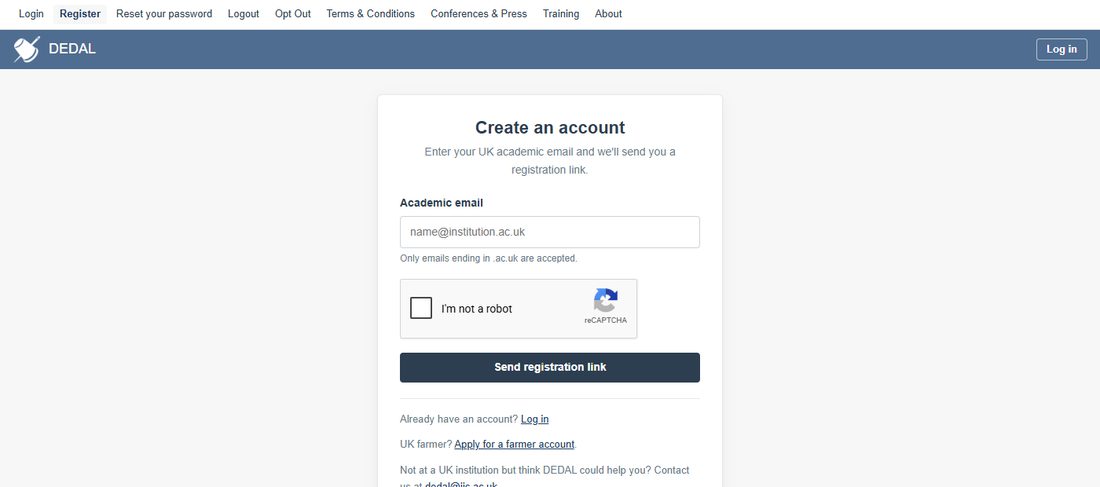
UK academics: on Register, enter your .ac.uk email. We email you a link (valid for 24 hours) where you choose a username and password. UK farmers: apply for a farmer account; we email your login details once it is approved.

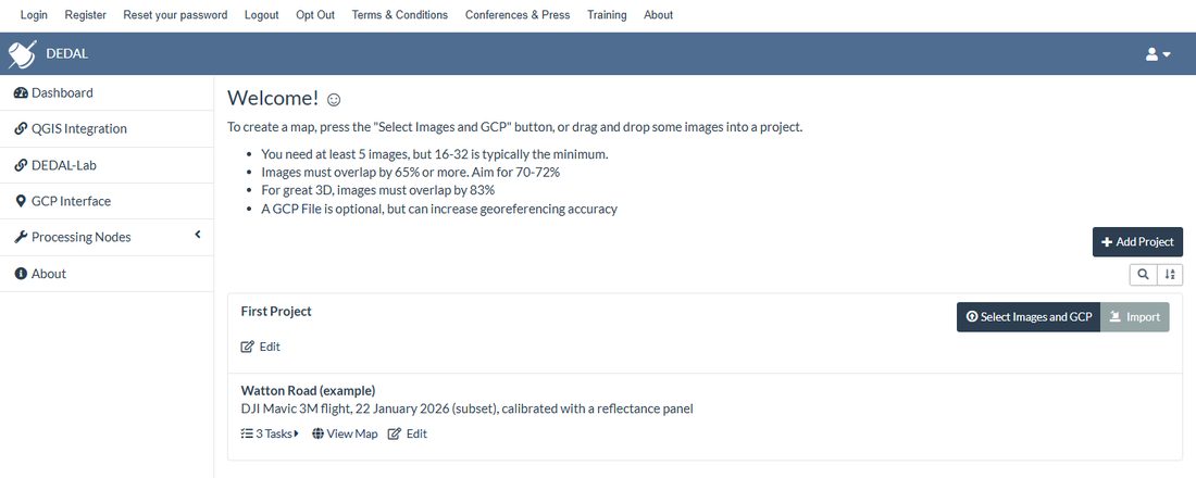
Then log in. Your dashboard lists your projects; each project holds the flights (tasks) you process.

2 Process a flight

1. In a project, click Select Images and GCP and choose the flight's images (or drag them onto the project). You need at least 5 images, and they must overlap by 65 % or more.
2. Check the Name, and leave Processing Node as it is.
3. Choose the processing Options. Default suits ordinary RGB photos. For DJI Mavic 3M multispectral flights, use the calibration below instead.
4. Click Review, then Start Processing. The images upload, and the task runs on the JIC cluster. A small flight takes minutes; a large one a few hours. You can close the page while it runs.

3 Calibrate multispectral images (DJI Mavic 3M)

Calibration turns the camera's raw values into reflectance, using a photo of a reflectance panel and the drone's sunlight sensor. Only calibrated values can be compared between flights and dates. How it works, its validation, and text for your methods section: Calibration method.

1. Include the panel shot. Select the flight's multispectral images (…_MS_G/R/RE/NIR.TIF) and the few images of the reflectance panel taken just before or after the flight. The RGB images (…_D.JPG) can be included; with calibration on, they are set aside.
2. Below the options, tick Calibrate to reflectance with a panel (DJI Mavic 3M). This sets everything calibration needs: the Panel pre-calibration (DJI Mavic 3M) options, and Resize Images: Yes, 100000 px, so that the images keep their full size.
3. Check the box's messages: Panel shot found among the images, and the panel used. The MicaSense RP04 panel is built in. If you use another panel, choose add a panel and enter its reflectance for green, red, red edge and NIR (from its certificate).
4. Review and Start Processing as usual.

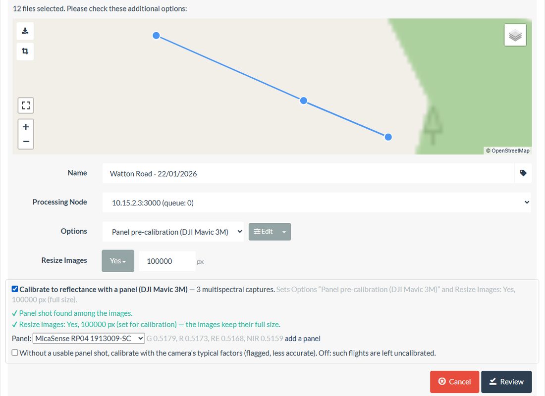
No panel shot? The flight is processed without calibration, unless you tick calibrate with the camera's typical factors. That gives an approximate calibration (about 5–6 % less accurate), which is flagged on the task.

Use your own panel

The default panel is the JIC's MicaSense RP04 (serial 1913009-SC). If you photograph a different panel, add it once and choose it from the Panel list; the panel you select is used for all your tasks.

1. In the calibration box, click add a panel.
2. Enter its name, and the reflectance for green, red, red edge and NIR from its calibration certificate, as fractions (0.49, not 49 %). Add its serial and certificate date too: they are recorded with every calibration, so results can be traced to the exact panel.
3. Save panel. It is selected straight away, and only you see it. Administrators can share a panel with everyone.

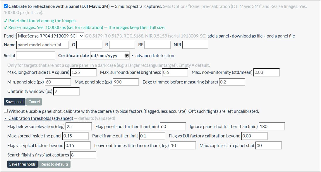
• Not a square panel in a dark case? Open advanced: detection. For example, a rectangular target twice as long as it is wide needs Max. long/short side of about 2.5. Leave the rest empty to keep the defaults.
• Share it, or use it on the JIC cluster: download as file saves the panel as a file; load a panel file adds a panel someone sent you. The cluster pipeline reads the same file, so the same panel gives the same result in both.
• Calibration thresholds (advanced) change the rules calibration follows, for example the sun elevation below which a result is flagged. The defaults were validated against Pix4D and across many flights. If you change them, your results are flagged as using custom thresholds, because they are no longer directly comparable with other calibrations. Reset to defaults undoes it.

4 Check the result

Open the project's tasks and click the task's name. When calibration ran, a line under the buttons says how it went:

• accepted: calibrated and passed every check;
• flagged: calibrated, with a warning to read, for example a low sun (below 25°) in winter flights;
• not calibrated: with the reason, for example no usable panel shot.

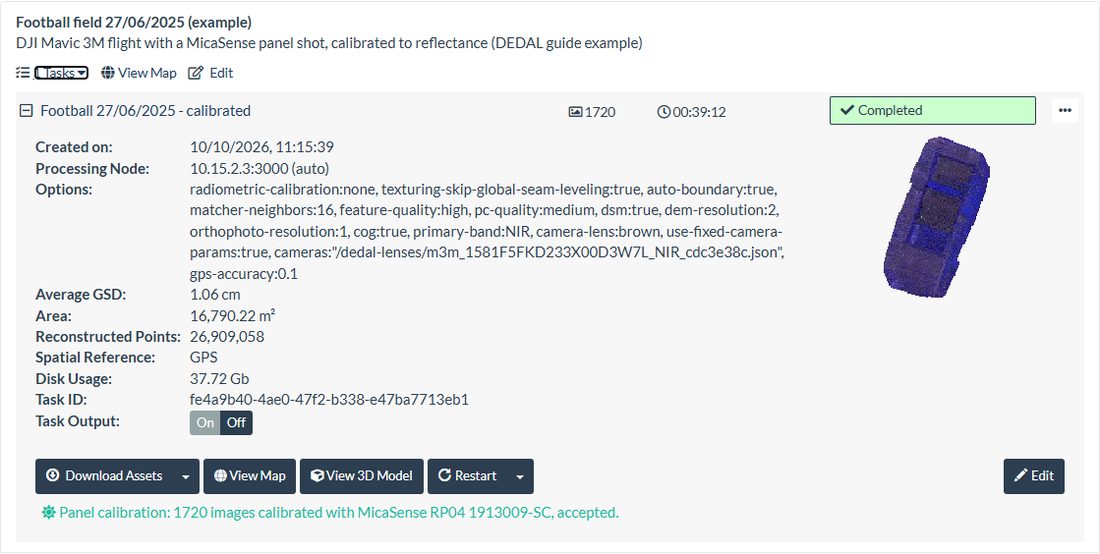
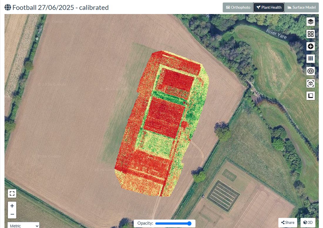
Click View Map to see the result. For multispectral flights the Orthophoto view looks dark, because reflectance values are small: use Plant Health for an NDVI map, or Surface Model for heights.

5 Extract plot data

DEDAL Extraction gives you a value per plot (for example the mean NDVI of each plot of a field trial) straight from the map, with nothing to install.

1. On the task's map, click the Plots button (the grid icon, top right). A panel opens with five steps.
2. Trial area. Click Draw trial area, then click the corner where plot 1 is, then the next corner along the direction the columns run, then the other corners, and Finish. It does not have to be exact: just keep neighbouring trials out. You can still drag and zoom the map while drawing. Already have your plots in a GIS? Use import a layout file instead (see below).

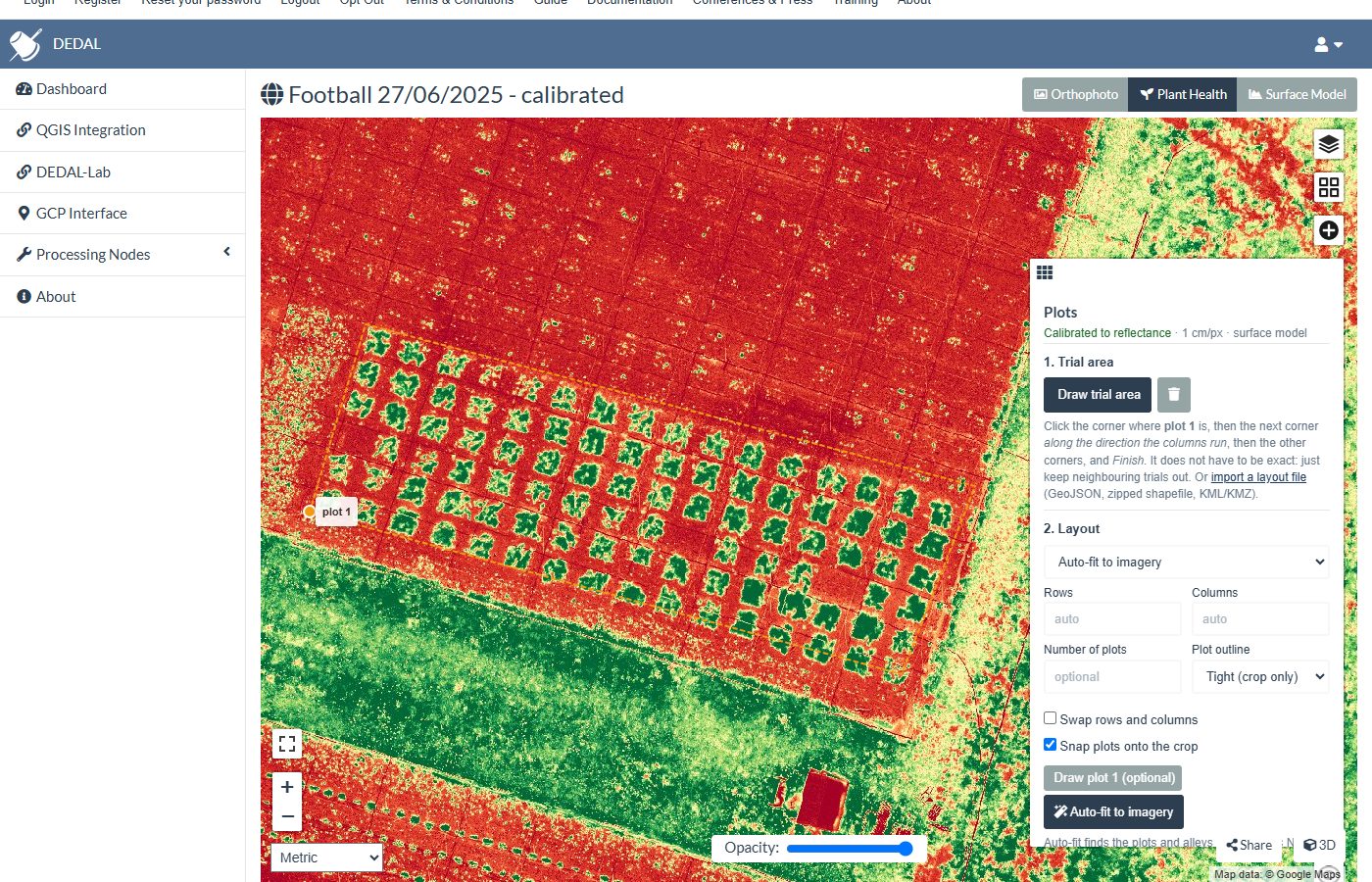
3. Layout. Choose how to make the plots, then press the button under it:
   • Auto-fit to imagery (the default) finds the plots and alleys in the flight's NDVI (or colours, for RGB flights) and reports the rows, columns, plot size and a quality: good, fair or poor. Leave rows and columns on auto, or type them, or the number of plots, if you know them. Snap plots onto the crop lets each plot move a little onto its own crop. If plot 1 is hard to find, Draw plot 1 to give its size and direction.
   • Fit to area: rows × columns spread over the area, with the gaps between plots in metres.
   • Fixed plot size: rows × columns of plots of a given width and length (metres), from plot 1's corner. Use it before the crop shows, when auto-fit has nothing to see.
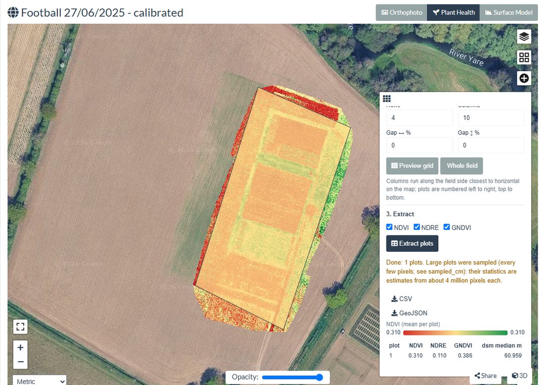
   • Whole field (one plot): the area itself as a single plot.
   The plots appear as a dashed preview.

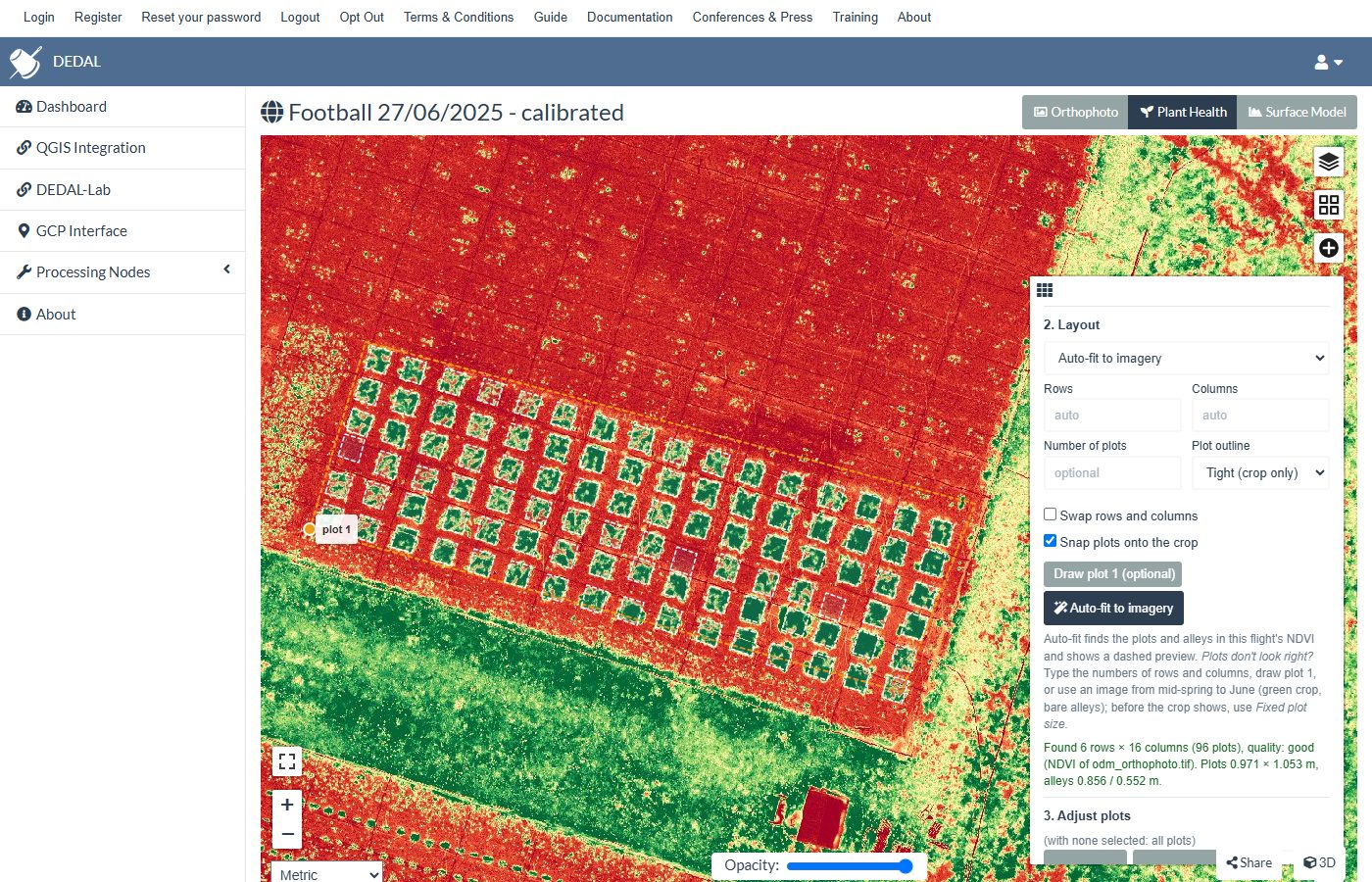
4. Adjust plots (if needed). Select plots and click them on the map (they turn yellow), then move them with the arrows, make them wider, narrower, longer or shorter in steps of 5 cm, 20 cm or 1 m, or remove them. With nothing selected, the buttons act on all plots.
5. Numbering. Plots are numbered row by row from plot 1 (prefix and first number of your choice, optionally serpentine). Load a plot sheet (CSV or Excel) to use your own plot codes: it is matched by row and column if it has them, otherwise in plot order, and its other columns (variety, treatment, rep, anything else) are added to the results. Tick labels to see the codes on the map.

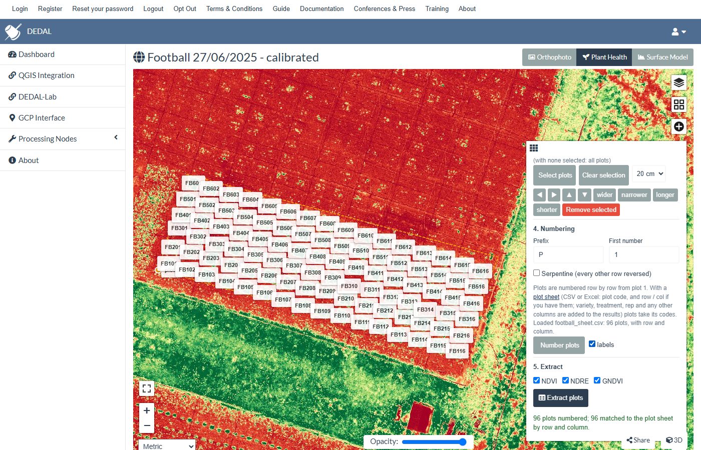
6. Extract. Choose the indices and click Extract plots.

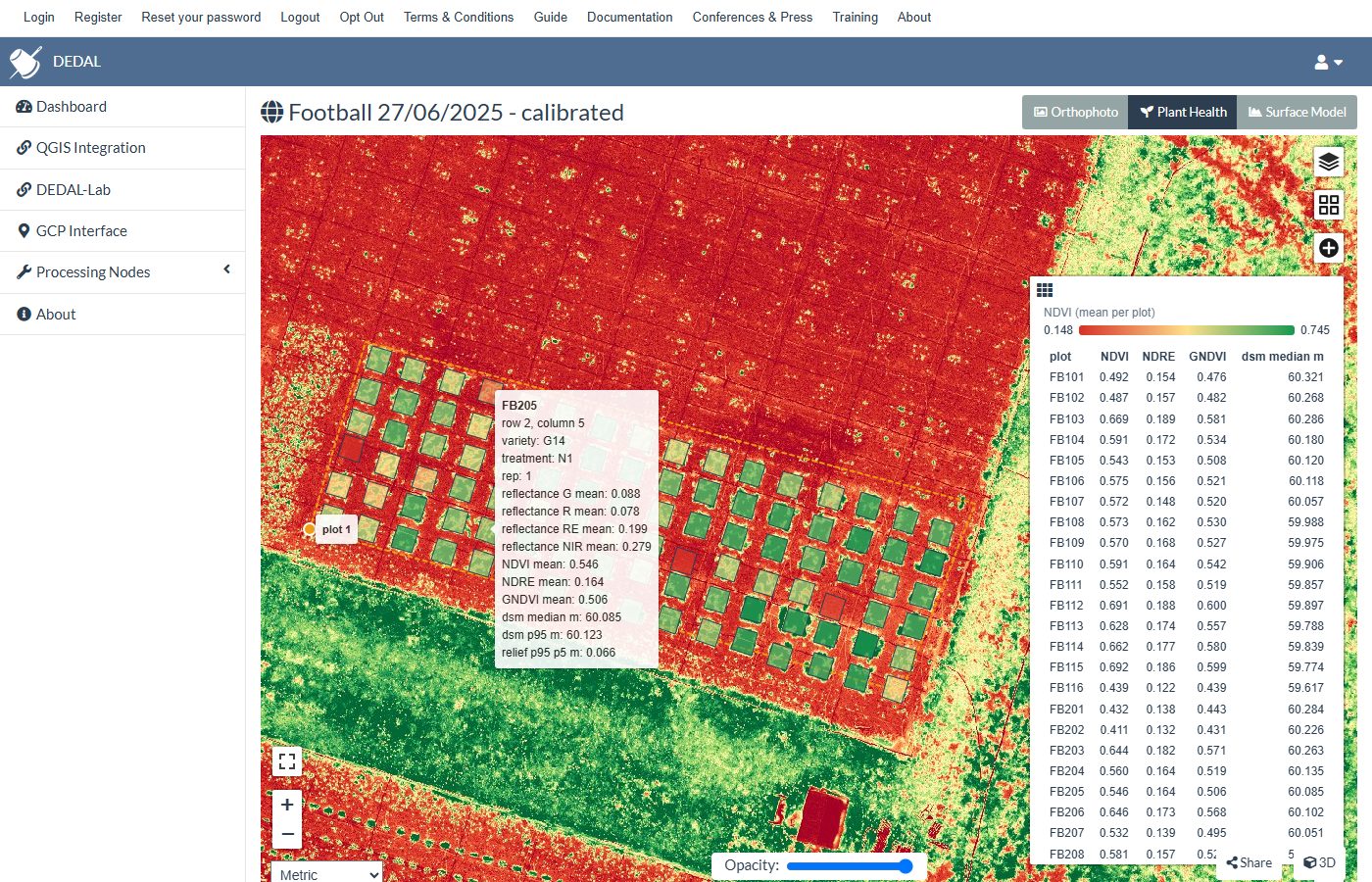
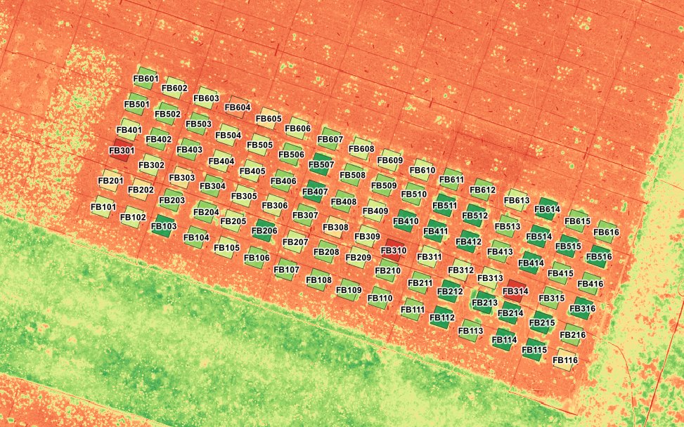
The plots are coloured from red (low) to green (high), with a table of the values in the panel. Hover over a plot to see all of its values, and download them with CSV (a table for Excel or R) or GeoJSON (the plots with their values, for GIS). Your plots are saved with the task and reappear the next time you open the panel.

What you get for each plot

• Multispectral flights: NDVI, NDRE and GNDVI (mean, median, standard deviation, minimum, maximum), and, when calibrated, the mean reflectance of each band. NDVI = (NIR − Red)/(NIR + Red), NDRE = (NIR − Red edge)/(NIR + Red edge), GNDVI = (NIR − Green)/(NIR + Green), the same as the DEDAL cluster pipeline.
• RGB flights: VARI, GLI and ExG.
• Surface model: the median and 95th percentile elevation, and the relief within the plot (95th − 5th percentile), a first estimate of canopy height.
• The plot's code, row, column, area and number of pixels, and the columns of your plot sheet or layout file. Pixels outside the flown area are left out.

Importing a layout

Import a layout file (step 1) loads plots you already have: GeoJSON, a zipped shapefile (.zip with the .shp, .shx, .dbf and .prj) or KML/KMZ, in any coordinate system (British National Grid included, converted with the Ordnance Survey's OSTN15 grid). The plot code is taken from a column such as plot, plot_code or label, and the other columns are kept. Point layouts (one point per plot) are not supported yet: use polygons.

6 Go further in DEDAL-Lab (R)

For analyses beyond the Plots panel (your own indices, soil removal and canopy cover, plant height, statistics and figures), DEDAL-Lab opens RStudio in your browser with the flight and your plots already in it, and a starter script.

1. Make and extract your plots (step 5), then click Go further in DEDAL-Lab under the downloads in the Plots panel. Or choose DEDAL-Lab in the menu and click Open in DEDAL-Lab next to the flight.
2. RStudio opens (the first time, after a short wait while the session starts). The flight is in flights/<flight name>/: the orthophoto, the surface model, your plots with their values and plot sheet columns, and analysis.R. Large orthophotos take a few minutes to copy; a COPYING.txt file is there until they are ready.
3. Open analysis.R and run it section by section (Ctrl+Enter). It works out NDVI, NDRE, GNDVI, OSAVI and CIre (VARI, GLI, ExG for RGB), separates crop from soil, and gives each plot its statistics, canopy cover and plant height (canopy top minus the ground in the alleys around the plot). Change the threshold, add indices or models: it is your copy.
4. The results are saved in results/: plots_lab.csv (your plot information plus the new values), plots_lab.gpkg for QGIS, and figures. Download them from the Files pane (tick → More → Export).

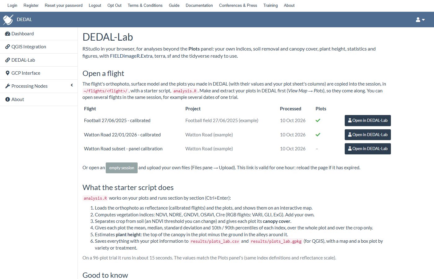
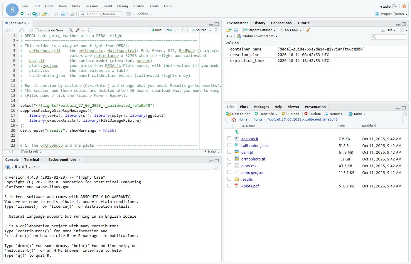
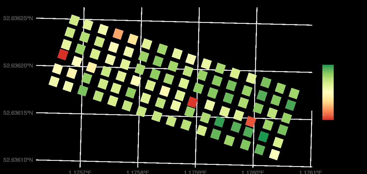
Open several flights in the same session (for example every date of a trial) to compare them: join the results by plot code. A session lasts 10 hours and is then deleted, with the copied flights.

7 Open a flight in QGIS

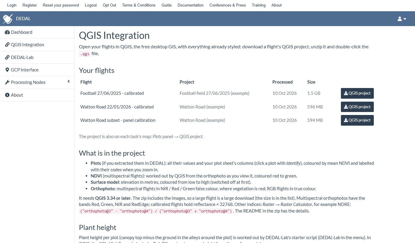
Every flight can be downloaded as a ready-made QGIS project (QGIS 3.34 or later, free): the orthophoto, NDVI, the surface model and your plots, already styled.

1. Click QGIS project at the top of the Plots panel, or choose QGIS Integration in the menu and click QGIS project next to the flight. Extract your plots first (step 5) so they come along.
2. Unzip the download and double-click the .qgs file. Keep the files of the folder together.

The plots are coloured by mean NDVI and labelled with their codes when you zoom in; click one with Identify to see all its values and your plot sheet's columns. NDVI is worked out by QGIS from the orthophoto as you view it. The orthophoto of a multispectral flight is shown in NIR / Red / Green false colour, where vegetation is red. The zip includes the images, so a large flight is a large download: the QGIS Integration page shows the size.

8 Download and good to know

• Download Assets on a task gives you the orthophoto, surface model, point cloud and report.
• Projects are deleted after 30 days (see the Terms and Conditions): download what you need.
• Questions or problems: dedal@jic.ac.uk.